Research note

Synaptic balance: from local rescaling to global order

On function-preserving changes of synaptic weights, local regularization, and the emergence of a unique balanced network.

Synaptic balance Local optimization Neural network symmetries Neuromorphic computing

A neural network's weights are not uniquely determined by the function it computes. Two networks can produce exactly the same outputs, for every input, while assigning very different magnitudes to their internal connections. This is particularly clear in networks with positively homogeneous activations, such as ReLU, where some changes to the incoming weights of a neuron can be compensated by opposite changes to its outgoing weights.

Normally, this freedom is treated as a property of the parameterization. In A theory of synaptic neural balance: From local to global order, Baldi and colleagues [1] use it to ask a different question: can neurons adjust their own synaptic weights, using only local information, so that the entire network approaches a well-defined configuration without changing its computation?

Their answer connects an elementary rescaling identity to a global convergence result. The interesting part is not that one neuron can be balanced. It is that balancing one neuron can disturb its neighbors, yet repeated local operations still converge to the same final weights.

A transformation that leaves the computation unchanged

Consider a hidden neuron whose activation function satisfies

$$\sigma(\lambda z)=\lambda\sigma(z),\qquad \lambda>0.$$

This positive homogeneity property holds for ReLU and leaky ReLU. More generally, the paper characterizes the scalar, degree-one homogeneous activations as bilinear units (BiLUs): functions with potentially different slopes on the positive and negative half-lines.

Suppose the neuron has incoming weights $w_{ij}$ and outgoing weights $w_{ki}$. Apply the transformation

$$w_{ij}'=\lambda w_{ij},\qquad w_{ki}'=\frac{w_{ki}}{\lambda}.$$

Any bias of the rescaled neuron must also be multiplied by $\lambda$. The neuron's activation is scaled by $\lambda$, but its contribution to downstream neurons is divided by the same factor. Consequently, the input–output function of the network is unchanged.

If the objective is separated into a task-dependent term and a weight regularizer,

$$\mathcal{L}(W)=E(W)+\alpha R(W),$$

then this operation leaves $E(W)$ unchanged while generally changing $R(W)$. It moves through different parameterizations of the same computation.

This distinction matters. A reduction in the regularizer obtained by rescaling does not, by itself, mean that the network has learned a better mapping. The mapping has not changed at all. Rescaling symmetries also motivate methods such as path-normalized optimization [3], although the balancing construction studied here has a different objective.

What does it mean for a neuron to be balanced?

Take a simple additive $L_p$ cost, with $p>0$,

$$R(W)=\sum_{w\in W}|w|^p.$$

For one hidden neuron $i$, define the contributions from its incoming and outgoing synapses as

$$A_i=\sum_{j\in\mathrm{IN}(i)}|w_{ij}|^p, \qquad B_i=\sum_{k\in\mathrm{OUT}(i)}|w_{ki}|^p.$$

Assume both are nonzero. Under the rescaling above, the part of the regularizer affected by this neuron becomes

$$R_i(\lambda)=\lambda^p A_i+\lambda^{-p}B_i.$$

The task error is constant along this direction. Minimizing the regularizer therefore gives

$$\lambda_i^*=\left(\frac{B_i}{A_i}\right)^{\!1/(2p)}.$$

After applying this scale factor,

$$A_i'=B_i'=\sqrt{A_iB_i}.$$

The neuron is now synaptically balanced: the $L_p$ costs of its incoming and outgoing connections are equal. In the $L_2$ case, this says that the squared Euclidean norms of the two weight vectors are equal.

The reduction in the local contribution to the regularizer is particularly simple:

$$\Delta R_i =A_i+B_i-2\sqrt{A_iB_i} =\big(\sqrt{A_i}-\sqrt{B_i}\big)^2\geq0.$$

Thus one balancing operation has two properties: it cannot increase the $L_p$ regularizer, and it does not change the network's input–output function. The paper extends the construction to broader additive regularizers, although the equation defining the optimum need not remain an equality of the two raw regularization costs in that general case [1].

There is also an important terminological distinction: this is not the usual biological balance between excitation and inhibition. It is a relationship between the magnitudes of a neuron's input and output synaptic weights.

Why local balance is not yet global balance

If neurons were isolated, the argument above would settle the problem. In a network, however, the outgoing weight of one neuron is also an incoming weight of another.

Suppose neurons $i$ and $j$ are connected. Balancing $i$ changes their shared connection. That can alter the incoming cost of $j$ and make $j$ unbalanced. Balancing $j$ in turn may undo the balance previously achieved at $i$.

It helps to separate two operations:

• Scaling: apply a specified positive multiplier to one neuron and its reciprocal to outgoing connections. Scaling operations commute.

• Balancing: choose the multiplier that minimizes the current local regularization cost. Balancing operations generally do not commute, because the optimal multiplier changes when neighboring weights change.

There is therefore no immediate reason why repeatedly balancing randomly selected neurons should settle down, let alone settle down to the same configuration regardless of the order of updates.

This is the central question addressed by the convergence analysis in [1]. If every eligible neuron is revisited indefinitely, the local balancing procedure converges, under the paper's assumptions, to a unique balanced set of weights within the rescaling family of the initial network. The same conclusion applies to appropriate deterministic schedules, including cyclic updates.

The qualifier is essential: the theorem does not say that all neural networks, or all training runs, converge to one universal set of weights. The unique endpoint is defined relative to a fixed initial weight configuration and the transformations that preserve its computation.

The hidden convex problem

The convergence result becomes easier to understand by describing all the local rescalings at once.

Assign a positive cumulative scale factor $\Lambda_i$ to each hidden neuron, with $\Lambda=1$ at the input and output units. A weight on a directed connection from neuron $j$ to neuron $i$ then has the form

$$w_{ij}'=w_{ij}\frac{\Lambda_i}{\Lambda_j}.$$

Introduce an edge variable

$$\ell_{ij}=\log\Lambda_i-\log\Lambda_j.$$

For an $L_p$ regularizer, the cost becomes

$$R(\ell)=\sum_{(j\to i)}|w_{ij}|^p e^{p\ell_{ij}}.$$

On the active connections, this is a strictly convex function of the edge log-scales. The allowable variables are not independent: along a path from an input to an output, the scale factors telescope, giving

$$\sum_{(j\to i)\in\pi}\ell_{ij}=0.$$

Directed cycles in recurrent architectures give analogous constraints. These relations are linear in the log-scales. The regularizer is therefore minimized over a linear, hence convex, set of admissible rescalings.

This provides the geometric reason for the unique endpoint: different schedules trace different paths through the same admissible set, but they are all reducing a cost with the same optimum. The network reaches global order without computing a global learning signal at each step.

There is a useful way to interpret the result. A homogeneous network admits many parameter vectors representing the same function. Balancing chooses a particular representative of that scaling-equivalence class: the one minimizing the selected regularizer. In that sense, it removes some arbitrariness from the weights without changing the computation they express.

A small numerical illustration

Consider a feedforward ReLU network with three inputs, two hidden layers of four and two neurons, and one linear output. Its weights are deliberately initialized with uneven magnitudes. No data are used for training, and no gradient updates are applied.

At each step, we select one hidden neuron and perform its exact $L_2$ balancing operation. We compare a cyclic schedule with a random schedule. The quantities we track are the total squared-weight cost,

$$R_t=\sum_{w\in W_t}w^2,$$

and the network's balance deficit,

$$D_t=\sum_{i\in\mathrm{hidden}} \left(A_i(t)-B_i(t)\right)^2.$$

The deficit is zero precisely when every hidden neuron is balanced. We also check the network's outputs on a fixed collection of inputs, which should remain unchanged up to numerical precision, and compare the final weight tensors obtained with the two update schedules.

using CairoMakie
using Random

# Three inputs -> four ReLU units -> two ReLU units -> one output.
W1_initial = [
     0.4  -1.3   0.8;
     1.6   0.7  -0.5;
    -0.9   0.3   1.2;
     0.5  -0.4   1.1
]
W2_initial = [
     0.8  -1.5   0.25   1.4;
    -0.6   0.45  2.0   -0.9
]
W3_initial = [1.8 -0.35]

X = randn(MersenneTwister(42), 3, 64)

function predict(W1, W2, W3, X)
    W3 * max.(W2 * max.(W1 * X, 0.0), 0.0)
end

reference = predict(W1_initial, W2_initial, W3_initial, X)

function diagnostics(W1, W2, W3)
    incoming = vcat(
        vec(sum(abs2, W1; dims = 2)),
        vec(sum(abs2, W2; dims = 2))
    )
    outgoing = vcat(
        vec(sum(abs2, W2; dims = 1)),
        vec(sum(abs2, W3; dims = 1))
    )
    regularizer = sum(abs2, W1) + sum(abs2, W2) + sum(abs2, W3)
    deficit = sum(abs2, incoming - outgoing)
    return regularizer, deficit
end

function run_balancing(schedule; steps = 300)
    W1 = copy(W1_initial)
    W2 = copy(W2_initial)
    W3 = copy(W3_initial)
    rng = MersenneTwister(7)

    R = zeros(steps + 1)
    D = zeros(steps + 1)
    R[1], D[1] = diagnostics(W1, W2, W3)

    for step in 1:steps
        neuron = schedule == :random ? rand(rng, 1:6) : mod1(step, 6)

        if neuron <= 4
            i = neuron
            A = sum(abs2, W1[i, :])
            B = sum(abs2, W2[:, i])
            lambda = (B / A)^(1 / 4)
            W1[i, :] .*= lambda
            W2[:, i] ./= lambda
        else
            i = neuron - 4
            A = sum(abs2, W2[i, :])
            B = sum(abs2, W3[:, i])
            lambda = (B / A)^(1 / 4)
            W2[i, :] .*= lambda
            W3[:, i] ./= lambda
        end

        R[step + 1], D[step + 1] = diagnostics(W1, W2, W3)
    end

    error = maximum(abs.(predict(W1, W2, W3, X) - reference))
    return R, D, error, (W1, W2, W3)
end

R_cyclic, D_cyclic, err_cyclic, W_cyclic = run_balancing(:cyclic)
R_random, D_random, err_random, W_random = run_balancing(:random)

println("Cyclic: final cost = ", R_cyclic[end],
        ", deficit = ", D_cyclic[end],
        ", max output error = ", err_cyclic)
println("Random: final cost = ", R_random[end],
        ", deficit = ", D_random[end],
        ", max output error = ", err_random)
weight_difference = maximum(
    maximum(abs.(W_cyclic[k] .- W_random[k])) for k in 1:3
)
println("Maximum difference between final weights = ", weight_difference)

# A single grayscale figure, with line styles encoding update schedules.
set_theme!(Theme(
    font = "TeX Gyre Termes",
    fontsize = 16,
    backgroundcolor = :white,
    Axis = (
        backgroundcolor = :white,
        xgridvisible = false,
        ygridvisible = true,
        ygridcolor = (:black, 0.10),
        ygridwidth = 0.7,
        topspinevisible = false,
        rightspinevisible = false,
        spinewidth = 1.0,
        xtickalign = 1,
        ytickalign = 1,
        xticksize = 5,
        yticksize = 5,
        titlesize = 19,
        titlealign = :left,
        xlabelsize = 16,
        ylabelsize = 16,
    ),
    Legend = (framevisible = false, labelsize = 14)
))

steps = 0:300
fig = Figure(size = (1160, 575), backgroundcolor = :white)
Label(fig[1, 1:2], "Convergence through local synaptic balancing",
      fontsize = 25, halign = :left, tellwidth = false)

ax1 = Axis(fig[2, 1],
    title = "A   Regularization cost",
    xlabel = "Local balancing operations",
    ylabel = "Squared-weight cost",
    xticks = 0:15:90)
lines!(ax1, steps, R_cyclic;
       color = :black, linewidth = 2.8, label = "Cyclic")
lines!(ax1, steps, R_random;
       color = :black, linewidth = 1.8, linestyle = :dash,
       label = "Random")
xlims!(ax1, 0, 90)
ylims!(ax1, 17.3, 24.0)
axislegend(ax1, position = :rt)

ax2 = Axis(fig[2, 2],
    title = "B   Relative balance deficit",
    xlabel = "Local balancing operations",
    ylabel = "Relative balance deficit",
    yscale = log10,
    xticks = 0:50:300,
    yticks = ([1.0, 1e-5, 1e-10, 1e-15, 1e-20],
              ["10⁰", "10⁻⁵", "10⁻¹⁰", "10⁻¹⁵", "10⁻²⁰"]))
# A display floor is required for plotting zero on a logarithmic axis.
# It does not alter the simulation or its reported deficits.
relative_cyclic = max.(D_cyclic ./ D_cyclic[1], 1e-20)
relative_random = max.(D_random ./ D_random[1], 1e-20)
lines!(ax2, steps, relative_cyclic;
       color = :black, linewidth = 2.8)
lines!(ax2, steps, relative_random;
       color = :black, linewidth = 1.8, linestyle = :dash)
xlims!(ax2, 0, 300)
ylims!(ax2, 1e-20, 2.0)

Label(fig[3, 1:2],
      "Illustrative 3–4–2–1 ReLU network  ·  Fixed weights, no task learning  ·  L₂ balancing",
      fontsize = 12, halign = :left, tellwidth = false)
colgap!(fig.layout, 44)
rowgap!(fig.layout, 20)

save("synaptic-balance-from-local-rescaling-to-global-order.svg", fig)
nothing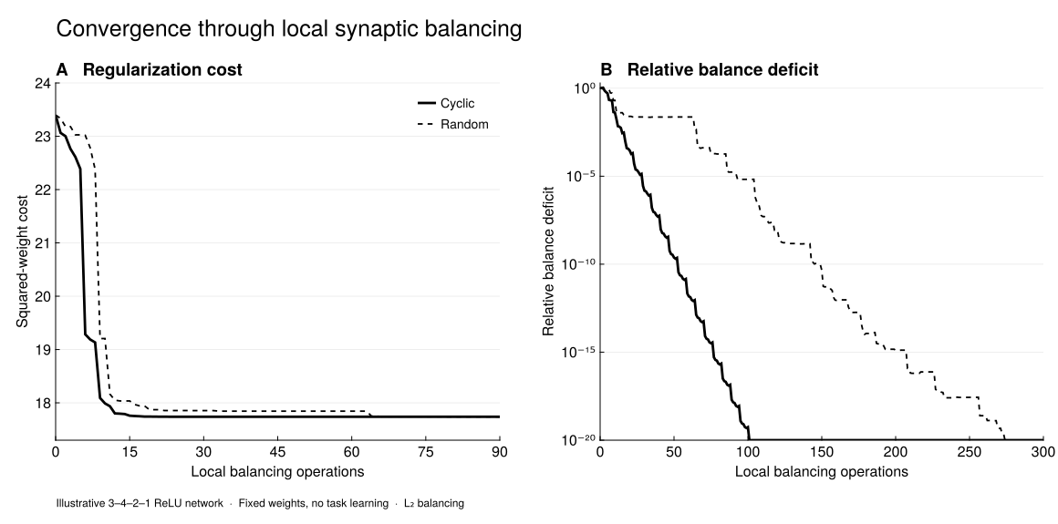

In this example the squared-weight cost decreases from about $23.4$ to $17.7$, while both schedules reduce the balance deficit to numerical precision. The top curve becomes almost flat before the lower curve has completely settled: an apparently stable regularizer is not, by itself, a proof that every neuron has finished balancing.

The plot is not an experiment on learning performance. It isolates the balancing dynamics from learning altogether. The reduction in $R_t$ is not a reduction in task error, and the convergence of $D_t$ does not imply that the network has become more accurate. It shows something narrower, but mathematically stronger: a sequence of neuron-local, function-preserving changes can converge to a common network-wide configuration.

Balance is a constraint on learning, not a substitute for it

The paper also distinguishes balancing algorithms from the balance that can arise during optimization of a regularized loss [1]. For degree-one homogeneous networks, continuous-time gradient flow on the unregularized task error preserves the difference between incoming and outgoing squared-weight costs [2]:

$$\frac{\mathrm d}{\mathrm dt}\left(A_i(t)-B_i(t)\right)=0 \qquad (p=2).$$

Thus, if the network is initially balanced, ideal gradient flow preserves that balance. This does not imply that finite-step gradient descent will do so, and it does not imply that training from an unbalanced initialization will eliminate the imbalance.

At a differentiable stationary point of a suitable regularized objective, the situation changes. If a neuron were unbalanced, one could rescale it to decrease the regularizer without affecting the task error, contradicting stationarity. Therefore balance is a necessary condition for such a stationary point. It is not sufficient: a perfectly balanced network can still have poor predictions, and balanced weights are not automatically an optimum of the task loss.

Baldi and colleagues also test balancing as a practical training operation. Their experiments include balancing before training and interleaving partial balancing with stochastic-gradient updates, with improvements in convergence and test performance on several feedforward and recurrent benchmarks [1]. Those findings are empirical and setting-dependent; they should not be confused with the theorem about the endpoint of balancing a fixed network.

Locality, biological plausibility, and the spiking case

The most attractive feature of this result for physical neural systems is its locality. A neuron needs information about its own incoming and outgoing synaptic costs, not the global loss or a backpropagated gradient. Nevertheless, local access to those quantities is a nontrivial physical requirement, and the paper does not establish that biological neurons actually implement this operation. Related work has studied synaptic balancing as a local mechanism for improving the noise robustness of recurrent networks [4], but its objective and analysis are not the same as the function-preserving regularizer minimization considered here.

It is tempting to transfer the result directly to spiking neural networks, but that requires care. ReLU-like homogeneity is a statement about how a neuron's output changes when its input is multiplied by a positive scalar. A spiking neuron with a firing threshold, reset, membrane time constant, and discrete output events does not generally satisfy the same identity. Rescaling its incoming and outgoing weights may change spike times or spike counts, even if a corresponding rate-based network would be unchanged.

There is also a hardware issue. Exact balancing uses continuous, reciprocal changes of synaptic weights. Discretized weights, finite weight ranges, and shared parameters can make that operation impossible or only approximate. Convolutional weight sharing presents a related difficulty in the paper itself: a rescaling that balances an individual neuron need not respect a shared kernel, so one may need coordinated, channel-level operations instead [1].

For spiking or neuromorphic systems, the principled extension would therefore start by identifying which transformations really preserve the relevant dynamics—the input–output map, a spike-based computation, or perhaps some weaker task-level observable—and only then asking whether a corresponding local regularizer can be minimized. Locality alone does not carry over the convergence or function-preservation guarantees.

That said, the paper suggests an interesting separation of roles. A task-dependent plasticity rule changes what the network computes. A balancing rule, when a suitable symmetry exists, changes how the same computation is represented in the synaptic weights. Those need not be the same operation or use the same information.

From local constraints to network structure

What I find most useful about synaptic balance is not the claim that input and output weight norms ought to match in every neural model. It is the more general construction: find a family of transformations that preserves a computation, define a local cost that distinguishes members of that family, and then ask whether iterating local reductions selects a stable global representation.

In Baldi et al., positive homogeneity supplies the invariance, the regularizer supplies the local objective, and convexity in logarithmic scaling coordinates explains why the final balanced representation is unique [1]. None of these ingredients alone gives the full result.

The broader question is whether other neuronal models admit similarly useful invariances, or sufficiently controlled approximations to them. For physical and event-driven networks, that seems more interesting than assuming that a weight-balancing rule can simply be imported unchanged. The central insight is that local organization can have a provable global consequence—even when the local operations interfere with one another.

References

1. P. Baldi, A. Alexos, I. Domingo, and A. Rahmansetayesh, “A theory of synaptic neural balance: From local to global order,” Artificial Intelligence, 346, 104360, 2025. doi:10.1016/j.artint.2025.104360

2. S. S. Du, W. Hu, and J. D. Lee, “Algorithmic regularization in learning deep homogeneous models: Layers are automatically balanced,” Advances in Neural Information Processing Systems, 31, 2018.

3. B. Neyshabur, R. R. Salakhutdinov, and N. Srebro, “Path-SGD: Path-normalized optimization in deep neural networks,” Advances in Neural Information Processing Systems, 28, 2015.

4. C. H. Stock, S. E. Harvey, S. A. Ocko, and S. Ganguli, “Synaptic balancing: a biologically plausible local learning rule that provably increases neural network noise robustness without sacrificing task performance,” PLOS Computational Biology, 18(9), e1010418, 2022. doi:10.1371/journal.pcbi.1010418