Research note
Fast and slow adaptation in a toy dynamical system
Many adaptive systems rely on processes that evolve at different speeds. Some components respond quickly to recent input, while others change more gradually and provide a more stable trace over time.
This distinction appears in several settings. In neuroscience, it suggests a rough analogy with short-term and longer-term memory processes. In learning systems, it relates to the tension between rapid adaptation and stability. In control or resource-constrained computation, it can shape how quickly a system reacts and how much of its past it preserves.
The small model below is not meant to be a biological theory of memory, nor a realistic learning architecture. It is only a minimal computational sketch that makes one idea visible: fast and slow processes can play different functional roles, even in a very simple dynamical system.
A simple intuition
If a system only adapts quickly, it can become highly responsive but also unstable or overly sensitive to short-term fluctuations.
If it only adapts slowly, it may be robust and smooth, but too sluggish to react to important changes.
A more interesting possibility is to let both dynamics coexist: a fast state, which reacts quickly to recent inputs, and a slow state, which integrates information more gradually.
Responsive and local
Moves quickly toward the current input and preserves a short-lived trace of recent changes.
Stable and cumulative
Changes more gradually, smooths fluctuations, and retains a steadier summary of recent history.
This is a very small abstraction, but it already suggests a useful interpretation: the fast state behaves like a short-lived trace of recent history, while the slow state behaves like a more stable accumulation over time.
That distinction is relevant well beyond neuroscience. It is a general design principle for adaptive systems.
The toy model
We consider an input signal x[t], together with two internal states: f[t], a fast variable, and s[t], a slow variable.
Both try to track the same input, but at different speeds. The update rule is deliberately simple:
f[t+1] = f[t] + eta_fast * (x[t] - f[t]) s[t+1] = s[t] + eta_slow * (x[t] - s[t]) with eta_fast > eta_slow
So the fast state moves quickly toward the current input, while the slow state changes more conservatively.
Julia sketch
using CairoMakie

T = 200
t = 1:T

# Input signal: a step followed by mild oscillations
x = [i < 50 ? 0.2 : 1.0 + 0.15*sin(0.15*i) for i in t]

fast = zeros(Float64, T)
slow = zeros(Float64, T)

η_fast = 0.25
η_slow = 0.03

for i in 2:T
    fast[i] = fast[i-1] + η_fast * (x[i] - fast[i-1])
    slow[i] = slow[i-1] + η_slow * (x[i] - slow[i-1])
end

fig = Figure(size = (850, 420))
ax = Axis(fig[1, 1], xlabel = "Time", ylabel = "State", title = "Fast and slow adaptation")
lines!(ax, t, x, label = "Input")
lines!(ax, t, fast, label = "Fast state")
lines!(ax, t, slow, label = "Slow state")
axislegend(ax, position = :rb)

save(joinpath(@OUTPUT, "fast-slow-toy-plot.png"), fig)
figWhat the toy system makes visible
The fast state stays much closer to the changing input, so it preserves responsiveness to short-term variation. The slow state lags behind and behaves more like a stabilizing trace.
That is the core intuition of the note: the same signal can support different computational roles once the update timescale changes.

What the model shows
Even in this minimal setup, the two variables behave differently in a useful way.
Reacts rapidly to changes in the input, tracks local variations more closely, and preserves short-term responsiveness.
Filters out fast fluctuations, changes more gradually, and preserves a more stable summary of recent history.
This does not yet give us “memory” in a strong cognitive sense. But it does show how different timescales can support different computational roles.
That is the main point.
A useful interpretation
One way to read this system is through a memory-oriented lens.
The fast variable can be interpreted as a rough analogue of a short-term adaptive trace: it is sensitive to what has happened recently and updates quickly when the environment changes.
The slow variable can be interpreted as a rough analogue of a longer-term stabilizing trace: it does not react immediately to every fluctuation, but it accumulates information more persistently.
This analogy should not be pushed too far. The model is far too small to represent real biological memory processes. But as a computational picture, it is useful because it makes a simple idea explicit:
different timescales can support different forms of retention, adaptation, and stability.
Why this matters for learning systems
This distinction becomes more interesting when we move from toy dynamics to adaptive models.
May help a system react to new inputs or contexts, adapt online, and remain sensitive to recent changes.
May help stabilize useful structure, preserve information over longer periods, and reduce destructive overwriting or forgetting.
That is why multi-timescale thinking appears naturally in discussions of continual learning, memory, meta-learning, neuromorphic systems, and adaptive intelligence under constraints.
The same general question keeps returning:
what should change quickly, and what should change slowly?
That is not just a neuroscience question. It is also an architectural and systems question.
Relation to neuroscience, without overstating it
Neuroscience provides part of the motivation here because it is hard to think about intelligence without thinking about memory, temporal integration, and plasticity across timescales.
But the main reason I find this useful is computational, not metaphorical. Multi-timescale organization gives a language for building systems that are both responsive and stable.
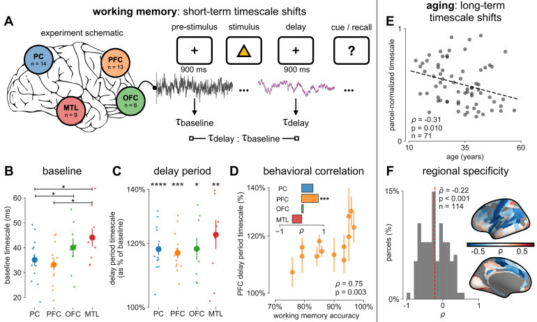
Two figures from Gao et al. are useful here because they connect neuronal timescales to measurable cortical organization without forcing a one-to-one mapping onto the toy system above.
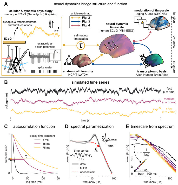
In that sense, the neuroscientific analogy is helpful not because it proves anything, but because it points toward a family of mechanisms where recent signals matter, older structure is not discarded immediately, and adaptation is distributed rather than uniform.
What this toy model does not capture
It is also important to say what is missing.
This toy system does not include recurrent structure, explicit plasticity rules, task-dependent modulation, memory retrieval, prediction or error-driven learning, or richer interactions between fast and slow processes beyond simple parallel tracking.
So it should be read only as a minimal sketch, not as a model of cognition or a serious theory of memory.
Why I still like it
I like examples like this because they are small enough to understand completely, but still rich enough to reveal a useful design principle.
The principle is simple:
adaptive systems do not need to change at one single speed.
Once that becomes visible, many further questions open up.
Possible next steps
Natural extensions would be to couple the fast and slow variables instead of updating them independently, add a modulatory signal that changes the update rates, use a nonstationary or task-switching input signal, interpret the variables as different forms of plasticity or memory traces, and connect the model to predictive or error-driven dynamics.
Closing thought
What interests me most here is not the toy model itself, but the broader idea behind it. Short-lived and longer-lived processes often need to coexist. Whether we call them fast and slow adaptation, short-term and long-term traces, or rapid plasticity and consolidation, the underlying computational question remains the same:
how can a system stay responsive to the present without losing too much of its past?