Research note

Fast adaptation and selective consolidation

A conceptual note on multi-timescale plasticity, familiarity, and the transition from transient adaptation to persistent memory.

Continual learning Multi-timescale plasticity Spiking neural networks Memory consolidation

Learning continuously is not only a problem of acquiring new information. It is also a problem of deciding which changes should last. A system that adapts rapidly can follow a changing environment, but the same plasticity that makes it responsive also makes it vulnerable to interference. A system that changes only slowly is more stable, but may fail to track short-lived structure that is nevertheless useful in the moment. This tension is closely related to the classical stability–plasticity problem, and it also appears in theoretical models of synaptic memory, where multiple internal states or timescales can substantially extend memory lifetime [1,2]. The interesting case is therefore not simply “fast learning versus slow learning”. It is what happens when the two coexist.

Fast and persistent components

A minimal abstraction is to write an adaptive state as the sum of a labile component and a persistent one,

$$w_t = w_t^{F} + w_t^{P}.$$

The fast component can react strongly to recent evidence and can also decay,

$$w_{t+1}^{F} = (1-\lambda_F) w_t^{F} + \eta_F u_t.$$

where $u_t$ is the update induced by the current observation. If the persistent component simply receives a smaller version of the same update,

$$w_{t+1}^{P} = w_t^{P} + \eta_P u_t, \qquad \eta_P \ll \eta_F.$$

then the model has two timescales, but not yet a mechanism for deciding what deserves long-term storage. Every fluctuation eventually leaks into the slow state. The timescale changes, but the selectivity problem remains. A more useful abstraction is

$$w_{t+1}^{P} = w_t^{P} + \eta_P g_t u_t.$$

where $g_t$ expresses whether the current modification is supported by enough evidence to become persistent. This distinction is close in spirit to ideas from metaplasticity and synaptic consolidation. Metaplastic changes can alter the future susceptibility of a synapse to plasticity without immediately changing its expressed efficacy [3]. Synaptic tagging and capture similarly separates the induction of a transient local state from the later stabilization of a long-lasting modification [4]. The computational question is analogous: an update can be available without immediately being committed.

Familiarity is not the memory itself

One way of thinking about $g_t$ is through familiarity. Here familiarity does not mean an explicit lookup saying that a particular sample has been seen before. It is better understood as a dynamical estimate that the current activity belongs to a structure that has been encountered repeatedly. A generic trace can be written as

$$m_{t+1} = (1-\beta)m_t + \beta \phi_t.$$

where $\phi_t$ is instantaneous evidence of recurrence or compatibility with previously established dynamics. In the simplest toy system, $\phi_t$ could be related to the distance between a fast state and a slower reference,

$$\phi_t = \exp\left(-\frac{\lVert f_t - s_t \rVert^2}{\tau^2}\right).$$

That equation is not meant as a final definition. Its role is only to make one point explicit: familiarity is a state accumulated through time, not the same thing as an individual prediction error and not the same thing as the stored content. This separation matters. A familiar input does not necessarily require a new memory update, and a large error does not necessarily indicate that something should be remembered. A volatile regime can generate strong and repeated errors while still being a poor candidate for persistent storage. Conversely, a recurring regime can become increasingly predictable while still providing evidence that a particular representation should be stabilized. Recent theoretical work on recall-gated consolidation develops a closely related principle: long-term learning can be protected from noisy updates by giving priority to changes that are consistent with what a short-term system recalls on later encounters [5]. The broader implication is that the decision to consolidate can depend on recurrence, rather than only on the magnitude of an instantaneous learning signal.

A small dynamical picture

The original version of this note used the simplest possible fast/slow tracker. A slightly richer toy picture is more useful here. Imagine a stream containing a recurring regime, mixed with temporary excursions. A fast state follows most of these changes. A persistent state reacts much less to isolated deviations and changes primarily when recurrent evidence has accumulated. The plot below is illustrative rather than experimental: it only visualizes the separation between responsiveness and persistence.

using CairoMakie
T = 420
t = collect(1:T)
x = fill(0.15, T)
regimes = [(55, 105), (175, 225), (295, 345)]
for (a, b) in regimes
    x[a:b] .= 1.0
end
x[125:145] .= 1.45
x[245:265] .= -0.45
x .+= 0.035 .* sin.(0.11 .* t)
fast = zeros(Float64, T)
persistent = zeros(Float64, T)
familiarity = zeros(Float64, T)
gate = zeros(Float64, T)
phi = zeros(Float64, T)
phi[55:105] .= 0.20
phi[175:225] .= 0.75
phi[295:345] .= 1.00
eta_fast = 0.18
eta_persistent = 0.035
beta_familiarity = 0.035
for i in 2:T
    fast[i] =
        fast[i-1] +
        eta_fast * (x[i] - fast[i-1])
familiarity[i] =
    (1 - beta_familiarity) * familiarity[i-1] +
    beta_familiarity * phi[i]

gate[i] =
    clamp((familiarity[i] - 0.18) / 0.22, 0.0, 1.0)

persistent[i] =
    persistent[i-1] +
    eta_persistent * gate[i] * (x[i] - persistent[i-1])
end
set_theme!(
    Theme(
        fontsize = 15,
        font = "TeX Gyre Termes",
        backgroundcolor = :white,
        Axis = (
            backgroundcolor = :white,
            xgridvisible = false,
            ygridvisible = false,
            topspinevisible = true,
            rightspinevisible = true,
            spinewidth = 1.0,
            xtickalign = 1,
            ytickalign = 1,
            xminorticksvisible = true,
            yminorticksvisible = true,
            xticksize = 6,
            yticksize = 6,
            xminorticksize = 3,
            yminorticksize = 3,
        ),
        Legend = (
            framevisible = false,
            backgroundcolor = :transparent,
            labelsize = 13,
        )
    )
)
fig = Figure(size = (920, 640))
ax1 = Axis(
    fig[1, 1],
    ylabel = "State",
    title = "Fast adaptation and selective persistence",
    xticklabelsvisible = false,
    xticksvisible = false,
)
for (a, b) in regimes
    vspan!(ax1, a, b, color = (:black, 0.045))
end
lines!(
    ax1, t, x,
    color = :black,
    linewidth = 1.25,
    linestyle = :dot,
    label = "Input stream"
)
lines!(
    ax1, t, fast,
    color = :black,
    linewidth = 1.6,
    linestyle = :dash,
    label = "Fast state"
)
lines!(
    ax1, t, persistent,
    color = :black,
    linewidth = 2.2,
    linestyle = :solid,
    label = "Persistent state"
)
axislegend(
    ax1,
    position = :rt,
    orientation = :horizontal,
    patchsize = (32, 12),
)
ax2 = Axis(
    fig[2, 1],
    xlabel = "Time",
    ylabel = "Control signal",
    yticks = ([0.0, 0.5, 1.0], ["0", "0.5", "1"]),
)
for (a, b) in regimes
    vspan!(ax2, a, b, color = (:black, 0.045))
end
lines!(
    ax2, t, familiarity,
    color = :black,
    linewidth = 1.6,
    linestyle = :dashdot,
    label = "Familiarity"
)
lines!(
    ax2, t, gate,
    color = :black,
    linewidth = 2.0,
    linestyle = :solid,
    label = "Consolidation gate"
)
hlines!(
    ax2, [0.18],
    color = (:black, 0.45),
    linewidth = 1.0,
    linestyle = :dot,
)
axislegend(
    ax2,
    position = :lt,
    orientation = :horizontal,
    patchsize = (32, 12),
)
rowsize!(fig.layout, 1, Relative(0.64))
rowsize!(fig.layout, 2, Relative(0.36))
rowgap!(fig.layout, 12)
linkxaxes!(ax1, ax2)
xlims!(ax1, 1, T)
Label(
    fig[3, 1],
    "Shaded intervals denote repeated encounters with the same latent regime.",
    fontsize = 12,
    halign = :left,
    tellwidth = false,
)
save("selective-consolidation-toy.png", fig, px_per_unit = 2)
fig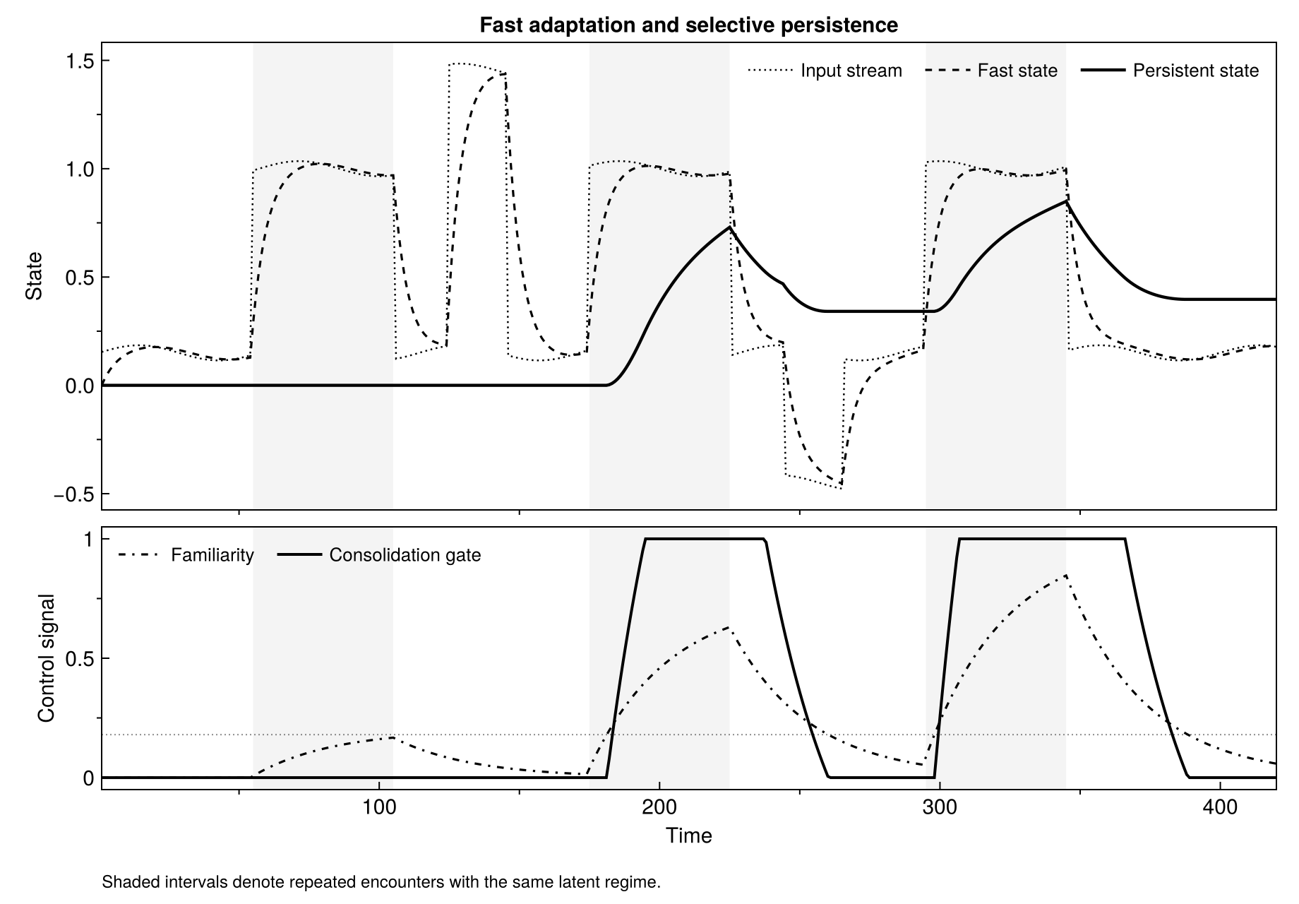

The plot is deliberately simple, but it highlights a distinction that tends to disappear when all adaptation is represented by a single set of weights. Fast plasticity answers what should change now?; consolidation answers which of those changes should still matter later?

Why a continuous stream changes the problem

This question becomes more interesting when there are no explicit task boundaries. In a task-based setup, a learner often knows that the distribution has changed because the experimental protocol tells it so. In a continuous stream, recurrence and change have to be inferred from the dynamics themselves. A regime may disappear and return after a long delay; stable structure can be interleaved with volatile structure; a transient deviation can resemble the beginning of a genuine distribution shift. Replay remains possible in such settings, but it solves part of the problem by keeping an explicit sample-level record of the past. A different question is what can be achieved when memory is carried primarily by the state and plasticity of the learner itself. This is one reason multi-timescale models are interesting. In the cascade model of Fusi, Drew and Abbott, and later in the framework of Benna and Fusi, long memory lifetimes arise from interactions among internal synaptic variables with different plasticity and retention properties [1,2]. The memory is not represented by repeatedly presenting stored examples; it is represented by the evolving state of the system. Selective consolidation adds another layer to that picture: the transition toward a slower state need not happen uniformly for every experience.

Why spiking systems are a natural substrate

The same idea becomes particularly natural in spiking neural networks because temporal state is already part of the model. A synapse can carry an eligibility-like trace,

$$e_{ij}(t)$$

produced by local pre- and postsynaptic activity. A modulatory signal $M_j(t)$ can then determine whether that local trace should induce a weight change,

$$\Delta w_{ij}(t) \propto M_j(t)e_{ij}(t).$$

This is the general structure of three-factor learning rules, which connect Hebbian or spike-timing-dependent eligibility with a third signal related to reward, novelty, error, or behavioral outcome [6,7]. Related ideas also appear in e-prop, where eligibility traces retain the part of the temporal gradient that can be computed locally in recurrent spiking networks, avoiding explicit backpropagation through the entire history [8]. A consolidation variable introduces an additional timescale,

$$\Delta w_{ij}^{P}(t) \propto g_j(t)M_j(t)e_{ij}(t).$$

The important point is not the extra multiplicative term by itself. It is the interpretation: the same event-driven machinery that supports online temporal credit assignment can, in principle, also support a slower decision about whether a modification remains labile or becomes persistent. Recent work has begun to explore related multi-timescale gating ideas directly in deep SNNs, for example by combining eligibility traces with a slower astrocyte-inspired plasticity gate [9]. This makes the distinction between a generic “slow learning rate” and a genuine slow state that regulates plasticity particularly relevant. The attraction of SNNs here is therefore not simply that spikes are biologically inspired. It is that several of the ingredients needed by the computational picture already have natural counterparts: membrane dynamics, synaptic traces, adaptive thresholds, sparse events, and local plasticity operating over different timescales.

From adaptation to memory

Seen this way, selective consolidation is not a particular network architecture. It is a way of organizing plasticity. The fast part of the system remains sensitive to recent evidence. A slower state accumulates information about recurrence or stability. Persistent plasticity is then allowed only when the two are consistent. One compact way to summarize the idea is

$$\underbrace{e_{ij}(t)}_{\text{local eligibility}} \;\times\; \underbrace{M_j(t)}_{\text{learning signal}} \;\times\; \underbrace{g_j(t)}_{\text{consolidation state}} \quad\longrightarrow\quad \text{persistent synaptic change}.$$

This resembles several ideas that already exist in neuroscience — metaplasticity, tagging, eligibility traces, multi-state synapses — without being identical to any one of them. The common theme is that a synaptic modification does not have to become permanent at the moment it is first induced. For continuous learning, that distinction is useful because the stream itself can provide evidence about what deserves persistence. Repetition, temporal consistency, low surprise, or agreement across encounters may all contribute to that evidence. The exact choice is model-dependent; the conceptual separation is not. In this view, forgetting is not only a failure to protect old information. Some forgetting is necessary. A useful adaptive system should be able to let transient changes disappear while allowing recurrent structure to move gradually onto a slower timescale. That is the computational role I find most interesting: not storing everything, but deciding what is allowed to last.

References

1. S. Fusi, P. J. Drew, and L. F. Abbott, “Cascade models of synaptically stored memories,” Neuron, 45(4), 599–611, 2005. doi:10.1016/j.neuron.2005.02.001

2. M. K. Benna and S. Fusi, “Computational principles of synaptic memory consolidation,” Nature Neuroscience, 19, 1697–1706, 2016. doi:10.1038/nn.4401

3. W. C. Abraham and M. F. Bear, “Metaplasticity: the plasticity of synaptic plasticity,” Trends in Neurosciences, 19(4), 126–130, 1996. doi:10.1016/S0166-2236(96)80018-X

4. R. L. Redondo and R. G. M. Morris, “Making memories last: the synaptic tagging and capture hypothesis,” Nature Reviews Neuroscience, 12, 17–30, 2011. doi:10.1038/nrn2963

5. J. W. Lindsey and A. Litwin-Kumar, “Selective consolidation of learning and memory via recall-gated plasticity,” eLife, 12:RP90793, 2024. doi:10.7554/eLife.90793

6. N. Frémaux and W. Gerstner, “Neuromodulated spike-timing-dependent plasticity, and theory of three-factor learning rules,” Frontiers in Neural Circuits, 9:85, 2016. doi:10.3389/fncir.2015.00085

7. W. Gerstner, M. Lehmann, V. Liakoni, D. Corneil, and J. Brea, “Eligibility traces and plasticity on behavioral time scales: experimental support of neoHebbian three-factor learning rules,” Frontiers in Neural Circuits, 12:53, 2018. doi:10.3389/fncir.2018.00053

8. G. Bellec et al., “A solution to the learning dilemma for recurrent networks of spiking neurons,” Nature Communications, 11, 3625, 2020. doi:10.1038/s41467-020-17236-y

9. Z. Dong and W. He, “Astrocyte-gated multi-timescale plasticity for online continual learning in deep spiking neural networks,” Frontiers in Neuroscience, 19:1768235, 2026. doi:10.3389/fnins.2025.1768235

10. J. Yik et al., “The NeuroBench framework for benchmarking neuromorphic computing algorithms and systems,” Nature Communications, 16, 1545, 2025. doi:10.1038/s41467-025-56739-4